Mini-Canister Hydrogen Transport
TMAP8 is used to model hydrogen transport and permeation through an aluminum-clad used nuclear fuel (AUNF) mini-canister storage device from Savannah River National Laboratory (SRNL) (d'Entremont and Verst, 2024). The mini-canisters house irradiated AUNF assemblies where gamma and neutron radiation from the fuel drives radiolytic decomposition of water, generating H gas. Over time, this hydrogen will dissociate and diffuse through the surrounding 304 stainless steel wall, raising concern for potential accumulation. This example demonstrates how TMAP8 can model these processes through two distinct input files with varying degrees of fidelity:
(test/tests/mini_canister/steel_only.i) — isolates hydrogen diffusion through the steel wall with an assumed boundary partial pressure. This simpler model permits verification against an analytical solution, assuming time-independent Dirichlet boundary conditions.
(test/tests/mini_canister/gas_steel.i) — simulates the full system: radiolytic H generation, gas-phase transport inside the canister, and simultaneous permeation through the steel wall. This model is compared against SRNL experimental measurements (d'Entremont and Verst, 2024).
Both models share the same 1D axisymmetric geometry and material parameters for the steel wall. The progression from (test/tests/mini_canister/steel_only.i) to (test/tests/mini_canister/gas_steel.i) illustrates the flexibility of TMAP8 in building complexity incrementally.
Canister Geometry and Mesh
Both models represent the canister as a 1D axisymmetric domain in cylindrical coordinates (, ), using coord_type = RZ with rz_coord_axis = Y so that the -axis is the radial direction. The canister (d'Entremont and Verst, 2024) is visualized in Figure 1 with dimensions listed in Table 1.
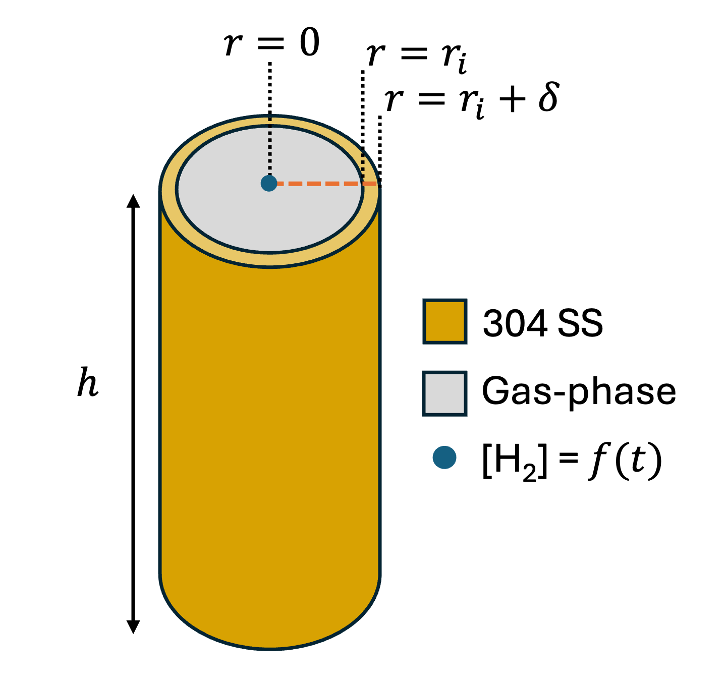
Figure 1: Schematic of SRNL mini-canister.
Table 1: Canister geometry.
| Parameter | Value | Units |
|---|---|---|
| Inner radius, | mm | |
| Steel wall thickness, | mm | |
| Canister height, | mm |
In (test/tests/mini_canister/steel_only.i), the 1D mesh spans only the steel wall, from to , using a single GeneratedMeshGenerator with 300 elements (subdomain 1). A bias is applied so that elements closer to the gas-steel boundary are smaller while elements further away are larger. In (test/tests/mini_canister/gas_steel.i), a CartesianMeshGenerator produces two adjacent blocks: the gas block (subdomain 0) from to with 25 elements, and the steel block (subdomain 1) from to with 300 elements. Two SideSetsBetweenSubdomainsGenerator steps then create the named interface sidesets interface_gas_to_steel and interface_steel_to_gas that are required for the ADInterfaceSorption / InterfaceSorption kernel.
In (test/tests/mini_canister/steel_only.i), the mesh is defined as:
[Mesh<<<{"href": "../../syntax/Mesh/index.html"}>>>]
  coord_type = 'RZ' # Axisymmetric coordinates
  rz_coord_axis = Y # Specifies X axis is radial direction and Y axis is axis of symmetry
  [steel]
    type = GeneratedMeshGenerator<<<{"description": "Create a line, square, or cube mesh with uniformly spaced or biased elements.", "href": "../../source/meshgenerators/GeneratedMeshGenerator.html"}>>>
    dim<<<{"description": "The dimension of the mesh to be generated"}>>> = 1
    nx<<<{"description": "Number of elements in the X direction"}>>> = ${num_elements_steel}
    xmin<<<{"description": "Lower X Coordinate of the generated mesh"}>>> = '${inner_radius}'
    xmax<<<{"description": "Upper X Coordinate of the generated mesh"}>>> = '${total_radius}'
    bias_x<<<{"description": "The amount by which to grow (or shrink) the cells in the x-direction."}>>> = 1.022
    subdomain_ids<<<{"description": "Subdomain IDs for each element, default to all zero. If a single number is specified, that subdomain id is used for all elements."}>>> = '1'
  []
[]
In (test/tests/mini_canister/gas_steel.i), the mesh is defined as:
[Mesh<<<{"href": "../../syntax/Mesh/index.html"}>>>]
  coord_type = 'RZ' # Axisymmetric coordinates
  rz_coord_axis = Y # Specifies X axis is radial direction and Y axis is axis of symmetry
  [cannister_radius]
    type = CartesianMeshGenerator<<<{"description": "This CartesianMeshGenerator creates a non-uniform Cartesian mesh.", "href": "../../source/meshgenerators/CartesianMeshGenerator.html"}>>>
    dim<<<{"description": "The dimension of the mesh to be generated"}>>> = 1
    dx<<<{"description": "Intervals in the X direction"}>>> = '${inner_radius} ${steel_thickness}'
    ix<<<{"description": "Number of grids in all intervals in the X direction (default to all one)"}>>> = '${num_elements_gas} ${num_elements_steel}'
    subdomain_id<<<{"description": "Block IDs (default to all zero)"}>>> = '0 1'
  []
  [interface_left]
    type = SideSetsBetweenSubdomainsGenerator<<<{"description": "MeshGenerator that creates a sideset composed of the nodes located between two or more subdomains.", "href": "../../source/meshgenerators/SideSetsBetweenSubdomainsGenerator.html"}>>>
    input<<<{"description": "The mesh we want to modify"}>>> = cannister_radius
    primary_block<<<{"description": "The primary set of blocks for which to draw a sideset between"}>>> = '0' # gas chamber
    paired_block<<<{"description": "The paired set of blocks for which to draw a sideset between"}>>> = '1' # steel wall
    new_boundary<<<{"description": "The list of boundary names to create on the supplied subdomain"}>>> = 'interface_gas_to_steel'
  []
  [interface_right]
    type = SideSetsBetweenSubdomainsGenerator<<<{"description": "MeshGenerator that creates a sideset composed of the nodes located between two or more subdomains.", "href": "../../source/meshgenerators/SideSetsBetweenSubdomainsGenerator.html"}>>>
    input<<<{"description": "The mesh we want to modify"}>>> = interface_left
    primary_block<<<{"description": "The primary set of blocks for which to draw a sideset between"}>>> = '1' # steel wall
    paired_block<<<{"description": "The paired set of blocks for which to draw a sideset between"}>>> = '0' # gas chamber
    new_boundary<<<{"description": "The list of boundary names to create on the supplied subdomain"}>>> = 'interface_steel_to_gas'
  []
[]
Nomenclature
Table 2 lists the variables and physical parameters used in this example with their units.
Table 2: Nomenclature of variables and physical parameters.
| Symbol | Description | Units |
|---|---|---|
| Mobile H atom concentration in steel | mol mm | |
| Mobile H molecule concentration in gas | mol mm | |
| Diffusivity of H in 304 stainless steel | mm day | |
| Diffusivity of H in He | mm day | |
| Solubility of H in steel (Sieverts' constant) | mol mm Pa | |
| Partial pressure of H | Pa | |
| Temperature (constant) | K | |
| Ideal gas constant | J K mol | |
| Volumetric H generation rate in gas | mol mm day | |
| Cumulative H yield in gas | mol | |
| Time | day |
Steel-Only Model
Governing Equations
In the steel-only model, only hydrogen transport within the steel wall is simulated. The governing equation is a 1D diffusion model:
(1)
where the diffusivity follows an Arrhenius temperature dependence (San Marchi and Somerday, 2012):
(2)
Because coord_type = RZ is set, MOOSE automatically applies the axisymmetric cylindrical weighting to the diffusion kernel.
Boundary Conditions
At the inner steel surface (), the hydrogen concentration is fixed by Sieverts' law using the EquilibriumBC boundary condition. An auxiliary variable H_partial_pressure_gas is first set by a FunctionAux at the inner boundary, and EquilibriumBC then enforces:
(3)
where the factor of 2 converts from molecular H equilibrium to atomic H concentration, and the solubility follows an Arrhenius dependence:
(4)
The H partial pressure is provided by a function selected via the pressure_function input parameter. A nonexhaustive set of implementations include: (1) a power-law fit to experimental SRNL pressure data (SRNL_pressure) calculated using a power-law least-squares fit, used as the default for comparison to data (see Figure 6 and Figure 5) and for the conservation-of-mass check (see Figure 2):
(5)
or (2) a constant value (constant_pressure) that can be selected to enable the diffusion-front verification against a closed-form analytical solution (see Figure 3):
(6)
which assumes 10% of the 24 psi He-backfilled canister pressure is attributable to H (d'Entremont and Verst, 2024; Hlushko et al., 2024).
At the outer steel surface (), hydrogen is released to the ambient environment, and the concentration is set to zero by a DirichletBC (defined in (test/tests/mini_canister/mini_canister_base.i)):
(7)
Solver
Because the steel-only problem is linear (constant diffusivity, linear Sieverts' BC), (test/tests/mini_canister/steel_only.i) uses solve_type = LINEAR for a direct LU factorization at each timestep. The simulation runs for 0.25 years (≈ 91.3 days) using a BDF2 time integration scheme equipped with an iterative timestepper IterationAdaptiveDT.
Model Parameters
Table 3 lists the steel-only model parameters and simulation conditions.
Table 3: Steel-only model parameters and simulation conditions.
| Parameter | Description | Value | Units | Reference |
|---|---|---|---|---|
| Diffusivity pre-exponential factor | m s | San Marchi and Somerday (2012) | ||
| Diffusivity activation energy | kJ mol | San Marchi and Somerday (2012) | ||
| Solubility pre-exponential factor | mol mm Pa | San Marchi and Somerday (2012) | ||
| Solubility activation energy | kJ mol | San Marchi and Somerday (2012) | ||
| Temperature | K | d'Entremont and Verst (2024) |
Results
Conservation of Mass
As an internal consistency check, the total hydrogen mass integrated over the steel domain (annular_cylinder_total_mass_steel) is compared against the time-integrated net diffusive flux across the inner and outer boundaries (annular_cylinder_time_integrated_flux). Both integrals are weighted for the axisymmetric cylindrical geometry and then scaled by the canister height to represent 3D mass in mol H. Figure 2 shows a two-panel conservation check. Before the accumulated H mass exceeds 1 percent of the total final hydrogen yield, absolute error is shown (top panel) to avoid noise from near-zero denominators at early times. Once the threshold is crossed, the relative percent difference between the two quantities, defined as is calculated. The metric is highly sensitive to the postprocessors' small values within the first few timesteps, but quickly converges to a small value.
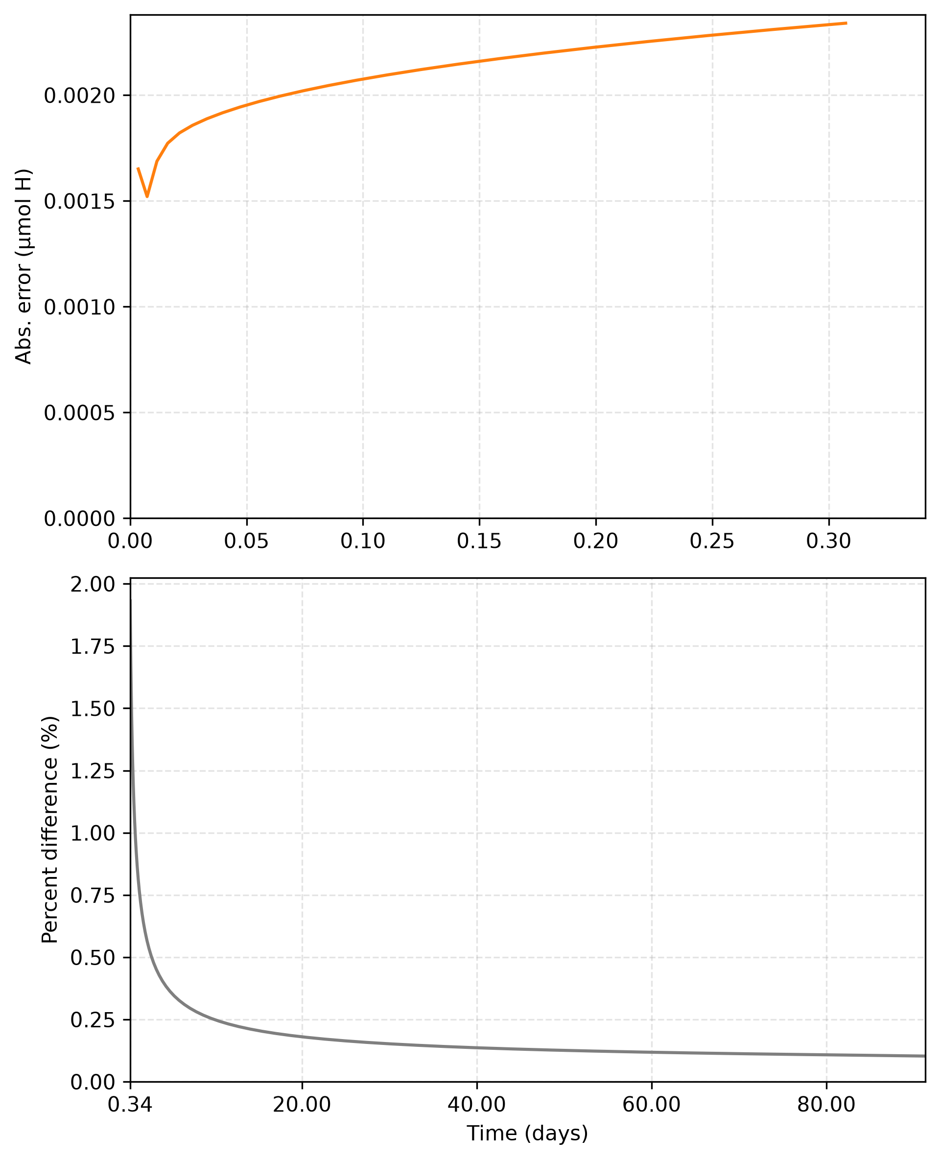
Figure 2: Conservation of mass for the steel-only model: percent difference . Absolute error is shown before the accumulated mass exceeds 1% of the total hydrogen yield (top); relative percent difference is shown thereafter (bottom).
Diffusion Front Verification
For a semi-infinite slab with a constant-concentration boundary condition, the diffusion front advances as , providing a straightforward check that the numerical diffusion is correctly implemented. The simulated diffusion front is computed via the simulated_diffusion_length postprocessor as the -intercept of the tangent line using the interface concentration and gradient. Figure 3 shows the simulated diffusion front length, using the constant pressure , compared to the analytical expression, which it matches.
In the input files, these two postprocessors are defined as:
[Postprocessors<<<{"href": "../../syntax/Postprocessors/index.html"}>>>]
  [exact_diffusion_length]
    # Analytical Diffusion length (time-independent BC required for this to be correct)
    type = ParsedPostprocessor<<<{"description": "Computes a parsed expression with post-processors", "href": "../../source/postprocessors/ParsedPostprocessor.html"}>>>
    expression<<<{"description": "function expression"}>>> = 'sqrt(pi*D*t)'
    constant_names<<<{"description": "Vector of constants used in the parsed function (use this for kB etc.)"}>>> = 'D pi'
    constant_expressions<<<{"description": "Vector of values for the constants in constant_names (can be an FParser expression)"}>>> = '${diffusivity_H_in_steel} 3.1415926535897932'
    use_t<<<{"description": "Make time (t) variable available in the function expression."}>>> = true
    outputs<<<{"description": "Vector of output names where you would like to restrict the output of variables(s) associated with this object"}>>> = csv
  []
[]
[Postprocessors<<<{"href": "../../syntax/Postprocessors/index.html"}>>>]
[simulated_diffusion_length]
# x-intercept of tangent line at interface
type = ParsedPostprocessor<<<{"description": "Computes a parsed expression with post-processors", "href": "../../source/postprocessors/ParsedPostprocessor.html"}>>>
expression<<<{"description": "function expression"}>>> = '-interface_concentration/gradient_left_boundary'
pp_names<<<{"description": "Post-processors arguments"}>>> = 'interface_concentration gradient_left_boundary'
outputs<<<{"description": "Vector of output names where you would like to restrict the output of variables(s) associated with this object"}>>> = csv
[]
[]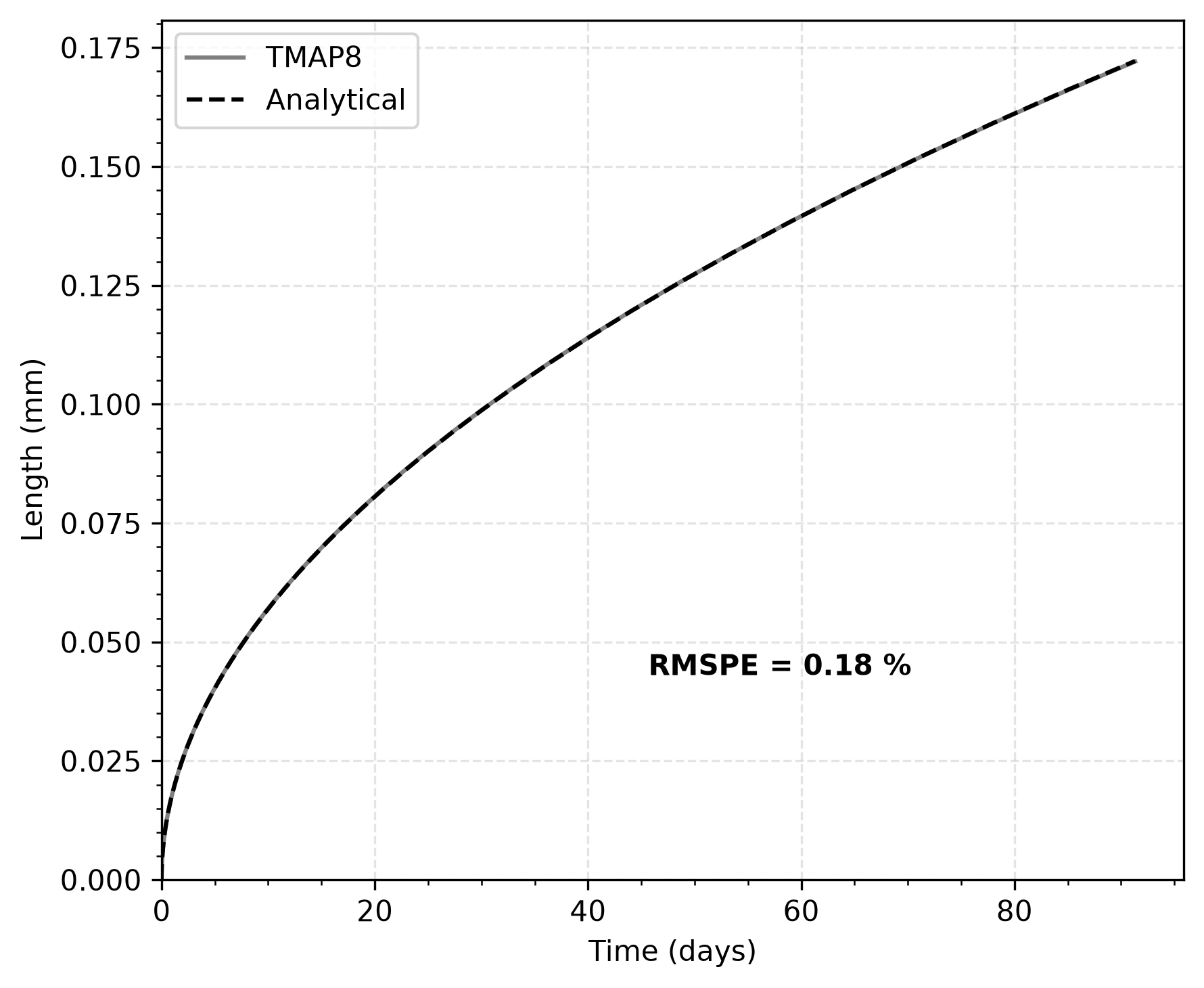
Figure 3: Comparison of the simulated and analytical () diffusion front length in the steel wall over 0.25 years.
Gas-Steel Model
Governing Equations
The gas-steel model resolves both the gas phase and steel simultaneously. In the gas phase (), H is generated by radiolysis and transported by diffusion:
(8)
where is the diffusivity of H in the He backfill gas (Middha et al., 2002). In the steel wall (), Eq. (1) applies as before. The axisymmetric weighting is again applied automatically by MOOSE. At the symmetry axis (), MOOSE's natural boundary condition enforces zero diffusive flux.
Hydrogen Generation Source Term
The cumulative radiolytic H yield is modeled using a power-law fit to the SRNL experimental data (d'Entremont and Verst, 2024), again calculated using a power-law least-squares fit:
(9)
where is time in days, calibrated assuming a Co-60 irradiator dose rate of approximately 124 Gy/min (d'Entremont and Verst, 2024). The volumetric source term in Eq. (8) is obtained by differentiating Eq. (9) with respect to time and normalizing by the gas volume:
(10)
Interface Condition
At the gas-steel interface (), hydrogen equilibrium between the gas and solid phases is enforced by the ADInterfaceSorption / InterfaceSorption interface kernel. Using the ideal gas law to convert gas-phase concentration to partial pressure (), the equilibrium atomic hydrogen concentration in the steel is:
(11)
The unit_scale_neighbor parameter is set to to correct for the unit mismatch between in mol mm and the ideal gas constant used internally by ADInterfaceSorption / InterfaceSorption, which draws in J K mol from the MOOSE PhysicalConstants namespace. Converting from mol mm to mol m introduces a combined factor of (mol/mol) (mm/m) , which is supplied via unit_scale_neighbor. The extra factor of converts the solubility to represent atomic .
Solver
Because the interface is nonlinear, (test/tests/mini_canister/gas_steel.i) uses solve_type = Newton. The simulation runs for 0.25 years (≈ 91.3 days) using a BDF2 time integration scheme. This model is equipped with an IterationAdaptiveDT adaptive timestep that targets 5 Newton iterations per step.
Model Parameters
Table 4 lists the parameters used in the gas-steel model.
Table 4: Additional gas-steel model parameters (steel parameters as in Table 3).
| Parameter | Description | Value | Units | Reference |
|---|---|---|---|---|
| H diffusivity in He | cm s | Middha et al. (2002) | ||
| Internal gas volume | mm | Computed |
Results
Conservation of Mass
Figure 4 verifies conservation of mass in the gas-steel model by comparing the total hydrogen mass in the gas and steel (cylinder_total_mass) against the sum of the time-integrated boundary flux (cylinder_time_integrated_flux) and the cumulative source term (cylinder_total_generation). Throughout, all quantities are tracked in mol H atoms. The figure plots the percent difference between the two quantities, defined as . Before the accumulated H mass exceeds 1 percent of the total final hydrogen yield, absolute error is once again shown (top panel) to avoid noise from near-zero denominators at early times. Once the threshold is crossed, the relative percent difference between the two quantities is calculated. The metric remains small, confirming that mass contributions from the coupled gas-generation, gas-phase transport, interface transfer, and steel diffusion are all consistently accounted for.
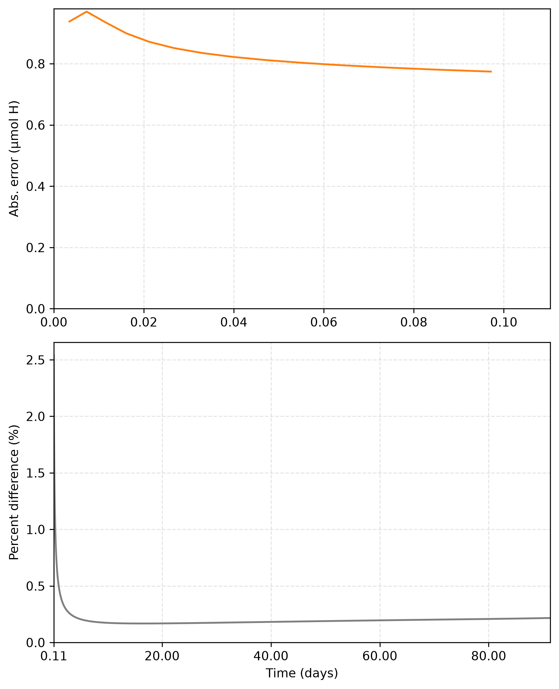
Figure 4: Conservation of mass for the gas-steel model: percent difference . Absolute error is shown before the accumulated mass exceeds 1% of the total hydrogen yield (top); relative percent difference is shown thereafter (bottom).
Gas-Phase Hydrogen Yield Calculations
Figure 5 compares the total atomic hydrogen mass in the gas phase (inner_cylinder_total_mass_gas) against the cumulative H yield measured by SRNL (d'Entremont and Verst, 2024). Agreement between the simulation and experiment reflects the accuracy of the power-law source model (Eq. (9)). It is important to note that the simulation results are compared against data that is fed into the model, which does not enable this effort to be considered a validation. Future work will include a more complex generation model independent of this data.
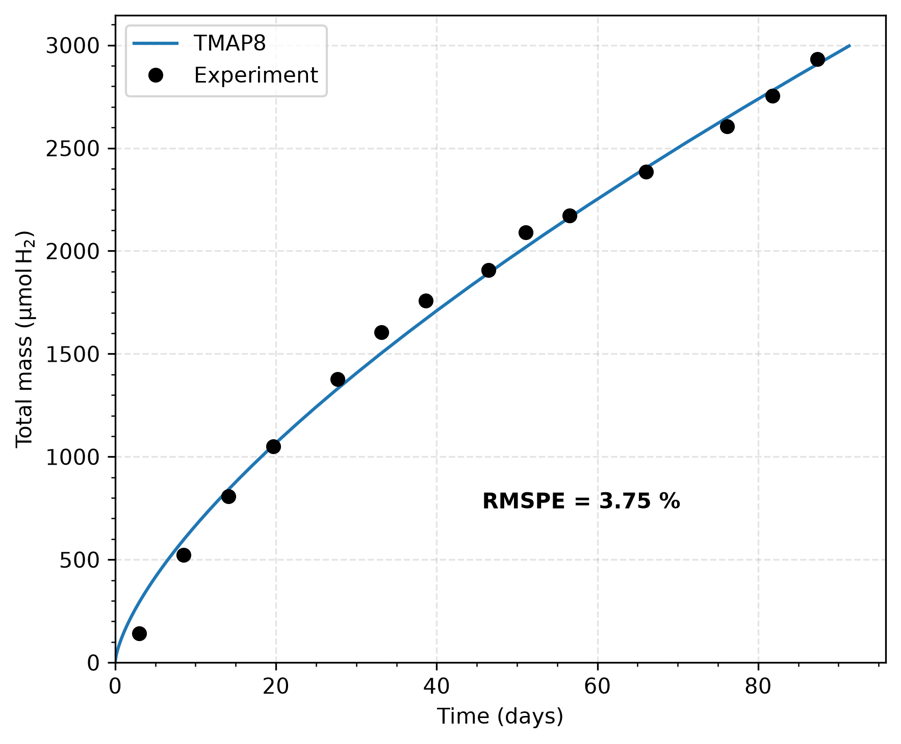
Figure 5: Comparison of TMAP8 total gas-phase hydrogen mass against SRNL experimental cumulative H yield data.
Partial Pressure Calculations
Figure 6 compares the simulated H partial pressure at the gas-steel interface against pressure measurements from the SRNL irradiation experiment (d'Entremont and Verst, 2024). The partial pressure is computed from the gas-phase concentration at the interface using the ideal gas law via the H_partial_pressure_interface postprocessor.
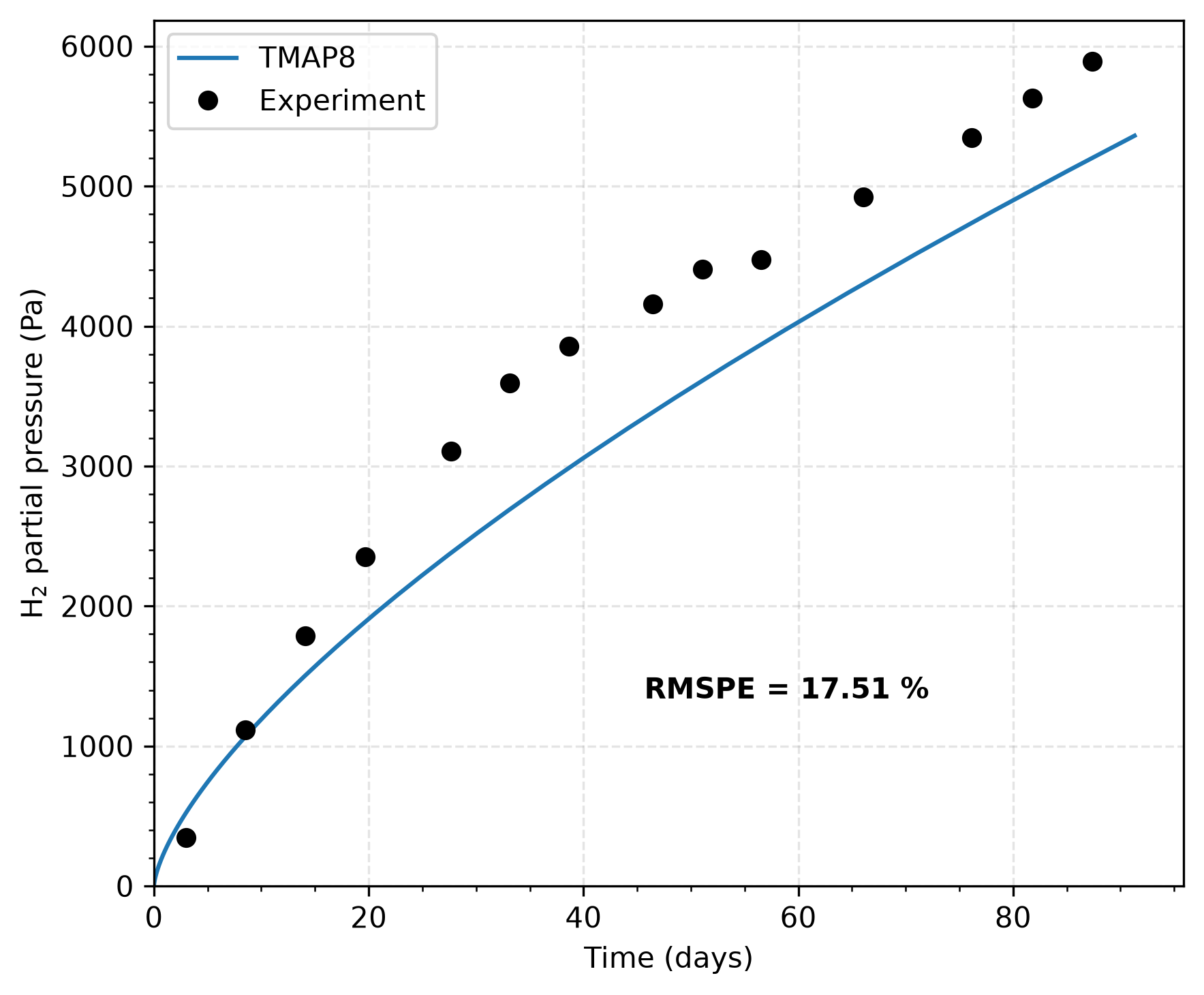
Figure 6: Comparison of TMAP8 simulated H partial pressure at the gas-steel interface against SRNL experimental measurements.
Comparison of Steel Hydrogen Uptake Between the Two Models
Figure 7 compares the total atomic hydrogen mass accumulated in the steel wall between the steel-only and gas-steel models. The left axis shows the absolute H mass in mol; the right axis shows the steel mass as a percentage of the total H inventory. By default the steel-only model uses the time-dependent SRNL partial-pressure fit (pressure_function = SRNL_pressure), giving decent agreement with the gas-steel model, which evolves the interface pressure self-consistently.
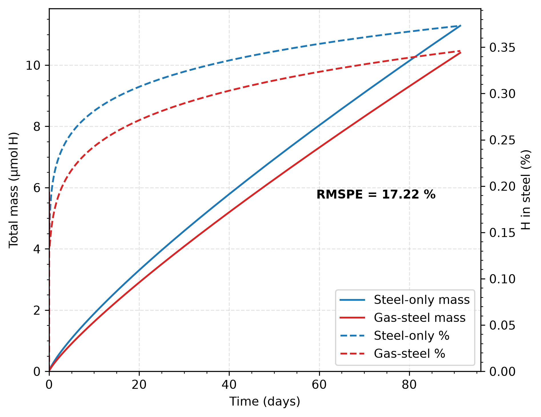
Figure 7: Comparison of total H mass in the steel wall (left axis) and fraction of total H inventory in the steel (right axis, dashed) between the steel-only (SRNL pressure fit) and gas-steel simulations.
The conclusion of this analysis is that only a small fraction of hydrogen permeates into the steel canister over the relevant time frame in these conditions. This observation is supported by both models.
Input File Structure
Both models are structured around two shared files that are incorporated via the !include capability:
(test/tests/mini_canister/mini_canister.params) — defines all shared model parameters (geometry, material properties, numerics).
(test/tests/mini_canister/mini_canister_base.i) — defines the MOOSE objects shared by both models: the steel variable and kernels, temperature auxiliary variable, outer Dirichlet boundary condition, steel-domain postprocessors, and the executioner.
Each top-level input file adds only the objects that are specific to its model. This structure keeps the shared physics in one place and avoids duplication.
Input Files
The input files for this example are (test/tests/mini_canister/steel_only.i) and (test/tests/mini_canister/gas_steel.i), together with the shared (test/tests/mini_canister/mini_canister_base.i) and (test/tests/mini_canister/mini_canister.params). All files are also used as tests in TMAP8 at (test/tests/mini_canister/tests).
### This is the base input file for the mini-canister example case, which is
### incorporated into steel_only.i and gas_steel.i using the `!include` feature
### This file is not designed to be run on its own

[Variables<<<{"href": "../../syntax/Variables/index.html"}>>>]
  [H_mobile_steel] # Mobile H atoms within steel
    block = '1'
  []
[]

[Kernels<<<{"href": "../../syntax/Kernels/index.html"}>>>]
  [steel_mobile_time]
    type = ADTimeDerivative<<<{"description": "The time derivative operator with the weak form of $(\\psi_i, \\frac{\\partial u_h}{\\partial t})$.", "href": "../../source/kernels/ADTimeDerivative.html"}>>>
    variable<<<{"description": "The name of the variable that this residual object operates on"}>>> = H_mobile_steel
    block<<<{"description": "The list of blocks (ids or names) that this object will be applied"}>>> = 1
  []
  [steel_mobile_diff]
    type = ADMatDiffusion<<<{"description": "Diffusion equation Kernel that takes an isotropic Diffusivity from a material property", "href": "../../source/kernels/MatDiffusion.html"}>>>
    variable<<<{"description": "The name of the variable that this residual object operates on"}>>> = H_mobile_steel
    diffusivity<<<{"description": "The diffusivity value or material property"}>>> = '${diffusivity_H_in_steel}'
    block<<<{"description": "The list of blocks (ids or names) that this object will be applied"}>>> = 1
  []
[]

[AuxVariables<<<{"href": "../../syntax/AuxVariables/index.html"}>>>]
    [T] # Temperature
    initial_condition<<<{"description": "Specifies a constant initial condition for this variable"}>>> = ${temperature}
  []
[]

[AuxKernels<<<{"href": "../../syntax/AuxKernels/index.html"}>>>]
  [constant_temperature]
    type = ConstantAux<<<{"description": "Creates a constant field in the domain.", "href": "../../source/auxkernels/ConstantAux.html"}>>>
    variable<<<{"description": "The name of the variable that this object applies to"}>>> = T
    value<<<{"description": "Some constant value that can be read from the input file"}>>> = '${temperature}'
  []
[]

[BCs<<<{"href": "../../syntax/BCs/index.html"}>>>]
  [steel_air_boundary] # Boundary of steel and outside environment
    type = DirichletBC<<<{"description": "Imposes the essential boundary condition $u=g$, where $g$ is a constant, controllable value.", "href": "../../source/bcs/DirichletBC.html"}>>>
    boundary<<<{"description": "The list of boundary IDs from the mesh where this object applies"}>>> = '1'
    value<<<{"description": "Value of the BC"}>>> = 0
    variable<<<{"description": "The name of the variable that this residual object operates on"}>>> = H_mobile_steel
  []
[]

[Postprocessors<<<{"href": "../../syntax/Postprocessors/index.html"}>>>]

  [annulus_concentration_steel] # Axisymmetric: 2D integral of annulus
    type = ElementIntegralVariablePostprocessor<<<{"description": "Computes a volume integral of the specified variable", "href": "../../source/postprocessors/ElementIntegralVariablePostprocessor.html"}>>>
    variable<<<{"description": "The name of the variable that this object operates on"}>>> = H_mobile_steel
    block<<<{"description": "The list of blocks (ids or names) that this object will be applied"}>>> = '1'
    outputs<<<{"description": "Vector of output names where you would like to restrict the output of variables(s) associated with this object"}>>> = none
  []

  [annular_cylinder_total_mass_steel]
    type = ScalePostprocessor<<<{"description": "Scales a post-processor by a value", "href": "../../source/postprocessors/ScalePostprocessor.html"}>>>
    value<<<{"description": "The postprocessor to be scaled"}>>> = annulus_concentration_steel
    scaling_factor<<<{"description": "The scaling factor"}>>> = '${height}'
    outputs<<<{"description": "Vector of output names where you would like to restrict the output of variables(s) associated with this object"}>>> = csv
  []

  [outer_edge_outflux]
    type = ADSideDiffusiveFluxIntegral<<<{"description": "Computes the integral of the diffusive flux over the specified boundary", "href": "../../source/postprocessors/SideDiffusiveFluxIntegral.html"}>>>
    boundary<<<{"description": "The list of boundary IDs from the mesh where this object applies"}>>> = '1'
    variable<<<{"description": "The name of the variable which this postprocessor integrates"}>>> = H_mobile_steel
    diffusivity<<<{"description": "The name of the diffusivity material property that will be used in the flux computation. This must be provided if the variable is of finite element type"}>>> = ${diffusivity_H_in_steel}
    outputs<<<{"description": "Vector of output names where you would like to restrict the output of variables(s) associated with this object"}>>> = none
  []
[]

[Executioner<<<{"href": "../../syntax/Executioner/index.html"}>>>]
  type = Transient
  scheme = bdf2
  dtmax = '${dt_max}'
  dtmin = '${dt_min}'
  dt = '${dt_start}'
  automatic_scaling = true
  petsc_options_iname = '-pc_type'
  petsc_options_value = 'lu'
  end_time = ${endtime}
  [TimeStepper<<<{"href": "../../syntax/Executioner/TimeStepper/index.html"}>>>]
    type = IterationAdaptiveDT
    dt = ${dt_start}
    optimal_iterations = 5
    growth_factor = 1.1
    cutback_factor_at_failure = .9
  []
[]

[Outputs<<<{"href": "../../syntax/Outputs/index.html"}>>>]
  csv<<<{"description": "Output the scalar variable and postprocessors to a *.csv file using the default CSV output."}>>> = true
[]
### This input file models the transport of H2 through only the steel wall of the mini_canister,
### using EquilibriumBC to model the interface between the gas chamber and steel
# Model parameters
!include mini_canister.params
# Geometry
total_radius = '${units ${fparse inner_radius + steel_thickness} mm}'
# Pressure implementation: constant_pressure | time_ramp_pressure | SRNL_pressure
pressure_function = 'SRNL_pressure'
# Percentage (%) estimation of H_2 content within He backfill to 24 psi
estimated_pressure_gas = '${units ${fparse 24*0.10} psi -> Pa}'
# Shared objects between two models
!include mini_canister_base.i
[Mesh]
coord_type = 'RZ' # Axisymmetric coordinates
rz_coord_axis = Y # Specifies X axis is radial direction and Y axis is axis of symmetry
[steel]
type = GeneratedMeshGenerator
dim = 1
nx = ${num_elements_steel}
xmin = '${inner_radius}'
xmax = '${total_radius}'
bias_x = 1.022
subdomain_ids = '1'
[]
[]
[AuxVariables]
[H_partial_pressure_gas] # Partial pressure of H_2 in internal gas chamber in Pa
[]
[]
[AuxKernels]
[pressure_aux]
type = FunctionAux
function = ${pressure_function}
variable = H_partial_pressure_gas
boundary = '0'
[]
[]
[BCs]
[gas_steel_boundary] # Species equilibrium condition between internal gas and steel wall
type = EquilibriumBC
Ko = '${solubility_preexponential_factor_in_steel}'
Ko_scaling_factor = 2 # Convert solubility to represent H atoms
boundary = '0'
activation_energy = '${solubility_activation_energy_in_steel}'
enclosure_var = H_partial_pressure_gas
variable = H_mobile_steel
temperature = T
p = 0.5 # Sieverts' Law
[]
[]
[Functions]
[constant_pressure] # Assumed
type = ConstantFunction
value = '${estimated_pressure_gas}'
[]
[time_ramp_pressure]
type = TimeRampFunction
initial_value = 0
final_value = '${estimated_pressure_gas}'
ramp_duration = '${units 3 h -> day}'
[]
[SRNL_pressure] # Power model linear least sqaures fit to Pa vs days
type = ParsedFunction
expression = '376.7588*t^0.6177'
[]
[]
[Postprocessors]
# Diffusion front verification
[exact_diffusion_length] # Analytical Diffusion length (time-independent BC required for this to be correct)
type = ParsedPostprocessor
expression = 'sqrt(pi*D*t)'
constant_names = 'D pi'
constant_expressions = '${diffusivity_H_in_steel} 3.1415926535897932'
use_t = true
outputs = csv
[]
[gradient_left_boundary] # dC_s/dx @ x = inner_radius
type = ADSideDiffusiveFluxAverage
boundary = '0'
variable = H_mobile_steel
diffusivity = 1
outputs = none
[]
[interface_concentration] # C_s @ x = inner_radius
type = SideAverageValue
boundary = '0'
variable = H_mobile_steel
outputs = none
[]
[simulated_diffusion_length] # x-intercept of tangent line at interface
type = ParsedPostprocessor
expression = '-interface_concentration/gradient_left_boundary'
pp_names = 'interface_concentration gradient_left_boundary'
outputs = csv
[]
# Conservation of mass: Accumulated flux
[interface_influx] # Influx at interface
type = ADSideDiffusiveFluxIntegral
boundary = '0'
variable = H_mobile_steel
diffusivity = ${diffusivity_H_in_steel}
outputs = none
[]
[annulus_flux_difference]
type = ParsedPostprocessor
expression = '-interface_influx - outer_edge_outflux' # negative sign on influx to account for outward normal vector direction
pp_names = 'interface_influx outer_edge_outflux'
outputs = none
[]
[annulus_time_integrated_flux]
type = TimeIntegratedPostprocessor
value = annulus_flux_difference
time_integration_scheme = TRAPEZOIDAL-RULE
outputs = none
[]
[annular_cylinder_time_integrated_flux]
type = ScalePostprocessor
value = annulus_time_integrated_flux
scaling_factor = ${height}
outputs = csv
[]
[]
[Executioner]
solve_type = LINEAR # Direct solve of linear system by LU factorization
[]
[Outputs]
file_base = 'steel_only_out_${pressure_function}'
[]
### This input file models the transport of H2 through both the gas chamber and
### steel wall of the mini_canister, using InterfaceSorption to model the
### interface between the gas chamber and steel

# Model parameters
!include mini_canister.params
# Volume of gas chamber in canister
gas_volume = '${units ${fparse pi*inner_radius^2*height} mm^3}'
# H2 diffusivity in He backfill
diffusivity_H2_in_He = '${units 2.7 cm^2/s -> mm^2/day}'
# Numerics
num_elements_gas = 25

# Shared objects between two models
!include mini_canister_base.i

[Mesh]
  coord_type = 'RZ' # Axisymmetric coordinates
  rz_coord_axis = Y # Specifies X axis is radial direction and Y axis is axis of symmetry
  [cannister_radius]
    type = CartesianMeshGenerator
    dim = 1
    dx = '${inner_radius} ${steel_thickness}'
    ix = '${num_elements_gas} ${num_elements_steel}'
    subdomain_id = '0 1'
  []
  [interface_left]
    type = SideSetsBetweenSubdomainsGenerator
    input = cannister_radius
    primary_block = '0' # gas chamber
    paired_block = '1' # steel wall
    new_boundary = 'interface_gas_to_steel'
  []
  [interface_right]
    type = SideSetsBetweenSubdomainsGenerator
    input = interface_left
    primary_block = '1' # steel wall
    paired_block = '0' # gas chamber
    new_boundary = 'interface_steel_to_gas'
  []
[]

[Variables]
  [H_mobile_gas] # Mobile H_2 gas inside canister
    block = '0'
  []
[]

[Kernels]
  [gas_mobile_time]
    type = ADTimeDerivative
    variable = H_mobile_gas
    block = 0
  []
  [gas_mobile_diff]
    type = ADMatDiffusion
    variable = H_mobile_gas
    diffusivity = '${diffusivity_H2_in_He}'
    block = 0
  []
  [gas_source]
    type = ADBodyForce
    variable = H_mobile_gas
    block = 0
    function = gas_generation_rhs_function
  []
[]

[InterfaceKernels]
  [Equilibrium_gas_to_steel]
    type = ADInterfaceSorption
    K0 = '${fparse 2 * solubility_preexponential_factor_in_steel}' # Convert solubility to represent H atoms
    boundary = interface_steel_to_gas
    Ea = '${solubility_activation_energy_in_steel}'
    neighbor_var = H_mobile_gas
    variable = H_mobile_steel
    temperature = T
    n_sorption = 0.5 # Sieverts' Law
    diffusivity = '${diffusivity_H_in_steel}'
    unit_scale_neighbor = 1e3 # Unit corrections for C_s = K*\sqrt{unit_scale_neighbor*C_g*R*T}
  []
[]

[Functions]
  [gas_generation_function] # Power model linear least sqaures fit to mumol vs days (assuming 124 Gy/min dosage rate from SRNL report)
    type = ParsedFunction
    expression = '69.7055*t^0.6808'
  []

  [gas_generation_rhs_function] # Take time derivative of gas_generation_function and divide by volume to get appropriate units for source term in concentration per unit time (mumol/mm^3/day)
    type = ParsedFunction
    expression = '69.7055*0.6808*t^(0.6808-1)/${gas_volume}'
  []
[]

[Postprocessors]

  # Conservation of mass: Total mass in domain

  [inner_circle_concentration_gas_molecular] # Axisymmetric: 2D Integral of inner circle Cross section
    type = ElementIntegralVariablePostprocessor
    variable = H_mobile_gas
    block = '0'
    outputs = none
  []

  [inner_circle_concentration_gas]
    type = ScalePostprocessor
    value = inner_circle_concentration_gas_molecular
    scaling_factor = 2 # Count H atoms
    outputs = none
  []

  [circle_concentration]
    type = SumPostprocessor
    values = 'inner_circle_concentration_gas annulus_concentration_steel'
    outputs = none
  []

  [inner_cylinder_total_mass_gas]
    type = ScalePostprocessor
    value = inner_circle_concentration_gas
    scaling_factor = '${height}'
    outputs = csv
  []

  [cylinder_total_mass]
    type = SumPostprocessor
    values = 'inner_cylinder_total_mass_gas annular_cylinder_total_mass_steel'
    outputs = csv
  []

  # Conservation of mass: Accumulated flux

  [center_influx] # Influx at the center of canister (Natural BC enforces 0)
    type = ADSideDiffusiveFluxIntegral
    boundary = '0'
    variable = H_mobile_gas
    diffusivity = ${diffusivity_H2_in_He}
    outputs = none
  []

  [circle_flux_difference]
    type = ParsedPostprocessor
    expression = '-2*center_influx-outer_edge_outflux' # Account for sign of outward normal vector
    pp_names = 'center_influx outer_edge_outflux'
    outputs = none
  []

  [circle_time_integrated_flux]
    type = TimeIntegratedPostprocessor
    value = circle_flux_difference
    time_integration_scheme = TRAPEZOIDAL-RULE
    outputs = none
  []

  [cylinder_time_integrated_flux]
    type = ScalePostprocessor
    value = circle_time_integrated_flux
    scaling_factor = ${height}
    outputs = csv
  []

  # Conservation of mass: H generation source term

  [cylinder_total_generation]
    type = FunctionValuePostprocessor
    function = gas_generation_function
    scale_factor = 2 # Count H atoms
    outputs = csv
  []

  # Pressure calculation

  [Mobile_gas_interface] # C_g at the gas-steel interface
    type = SideAverageValue
    boundary = 'interface_gas_to_steel'
    variable = H_mobile_gas
    outputs = none
  []

  [H_partial_pressure_interface] # Use ideal gas law to approximate pressure
    type = ScalePostprocessor
    value = Mobile_gas_interface
    scaling_factor = '${fparse ideal_gas_constant * temperature*1e9}' # J/mm^3 = 1e9 J/m^3 = 1e9 Pa
    outputs = csv
  []
[]

[Executioner]
  solve_type = Newton
  line_search = NONE
  nl_rel_tol = 1e-07
[]

[Outputs]
  file_base = 'gas_steel_out'
[]
References
- Anna L. d'Entremont and Christopher G. Verst.
Mini-Canister Radiolysis Testing of ASNF Materials and Surrogates.
Technical Report, Savannah River National Laboratory (SRNL), Aiken, SC (United States), 10 2024.
URL: https://www.osti.gov/biblio/2477665, doi:10.2172/2477665.[Export]
- Hanna Hlushko, Joseph Richard Wilbanks, Gregory Peter Holmbeck, Corey D. Pilgrim, Jacy Kathleen Conrad, and Elizabeth H Parker-Quaife.
Milestone 1.2.16. Reconciling the Impacts of Thermal Pretreatment on Radiation-Induced H2 Generation from Aluminum-Clad Spent Nuclear Fuel Surrogate Materials.
Technical Report, Idaho National Laboratory (INL), Idaho Falls, ID (United States), 08 2024.
URL: https://www.osti.gov/biblio/2478662.[Export]
- Prankul Middha, Benhui Yang, and Hai Wang.
A first-principle calculation of the binary diffusion coefficients pertinent to kinetic modeling of hydrogen/oxygen/helium flames.
Proceedings of the Combustion Institute, 29(1):1361–1369, 2002.
Proceedings of the Combustion Institute.
URL: https://www.sciencedirect.com/science/article/pii/S1540748902801675, doi:https://doi.org/10.1016/S1540-7489(02)80167-5.[Export]
- Christopher W San Marchi and Brian P Somerday.
Technical reference for hydrogen compatibility of materials.
Technical Report, Sandia National Laboratories, 09 2012.
URL: https://www.osti.gov/biblio/1055634, doi:10.2172/1055634.[Export]